# Packages
library(survival)
library(dplyr)

# Data
## Get data
data(cancer, package = "survival")

## Transform and select data
data_f <- lung %>%
    dplyr::select(-c(ph.ecog, ph.karno, pat.karno, meal.cal, wt.loss)) %>%
    dplyr::mutate(sex = if_else(sex == 1, "Male", "Female")) %>%
    dplyr::mutate_at(.vars = c("inst", "status", "sex"), .funs = as.factor)

# Plot8 Survival function
$$ % Basic sets/Variables
% Probability and statistics % % Linear algebra % Math functions % Distributions% Update symbols $$
To describe how probable it is for a person to survive until some time \(t\), we can utilize the concept of stochastic variables (see Chapter 2). The CDF (see Section 2.2) can be used to describe the probability that an event occurs prior to time \(t\) - \(\mathbb{P}\left(T \leq t\right)\). The CDF of the stochastic variable \(T\) is often referred to as the cumulative incidence function (CIF) and can be expressed as \[ \begin{aligned} F_T(t) &= \mathbb{P}\left(T \leq t\right) \\ &= \int_0^t h(u) \cdot S(u) \,\mathrm{d}u \end{aligned} \tag{8.1}\] where \(S\) is the survival function and \(h\) is the hazard function. However, in survival analysis the opposite is of interest - that a person has survived past time \(t\). Thus, the survival function can be defined as \[ \begin{aligned} S(t) &= 1 - F_T(t) \\ &= \mathbb{P}\left(T > t\right) = \int_t^\infty f_T(x) \,\mathrm{d}x \end{aligned} \] where \(F_T\) is the CIF and \(f_T\) the pdf of \(T\). One of the proporties of the survival function is that it is monotonically decreasing, i.e. \(S(t_2) \leq S(t_1)\) for all \(t_1 \geq t_2\).
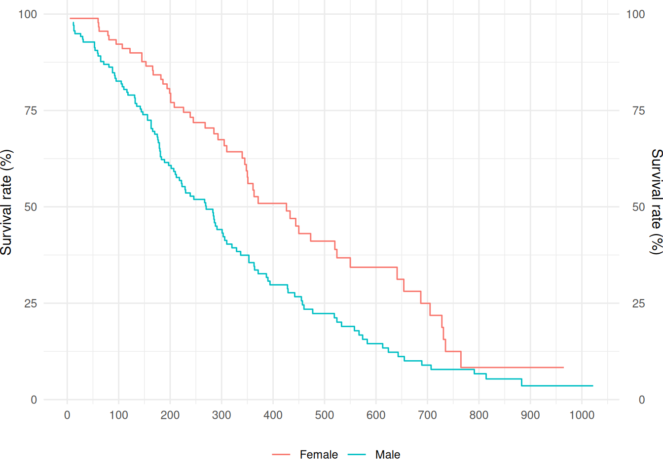
Example 8.1 (Survival Function)