Appendix A — Common Stochastic Variables
$$ % Basic sets/Variables
% Probability and statistics % % Linear algebra % Math functions % Distributions% Update symbols $$
A.1 Bernoulli
A bernoulli stochastic variable \(X\thicksim\operatorname{B}\left(n, p\right)\) has the sample space \(\Omega = \{0, 1\}\) with the probabilities \(\mathbb{P}\left(X = 1\right) = p\) and the opposite, \(\mathbb{P}\left(X = 0\right) = 1 - p\).
Distribution
\[ \begin{cases} p &\textrm{if } x = 1 \\ 1 - p &\textrm{if } x = 0 \end{cases} \]
Expected Value
\[ \mathbb{E}\left[X\right] = p \]
Variance
\[ \operatorname{Var}\left[X\right] = p \cdot (1 - p) \]
A.2 Binomial
A binomial stochastic variable is a Bernoulli stochastic variable repeated \(n\) times.
Distribution
The PMF (see Section 2.1) is given as \[ \binom{n}{k}\cdot p^k \cdot \left(1 - p\right)^{n - k} \] where \(k\) is the number of \(1\)’s out of the possible \(n\) experiments.
Expected Value
\[ \mathbb{E}\left[X\right] = n \cdot p \]
Variance
\[ \operatorname{Var}\left[X\right] = n \cdot p \cdot (1 - p) \]
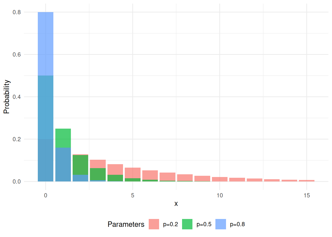
A.3 Geometric
The geometric distribution models the number of independent Bernoulli trials needed to obtain the first success, where each trial succeeds with probability \(p\). It is the discrete analogue of the exponential distribution and shares the memoryless property.
Distribution
Expected Value
\[ \mathbb{E}\left[X\right] = \frac{1}{p} \]
Variance
\[ \operatorname{Var}\left[X\right] = \frac{1 - p}{p^2} \]
A.4 Negative Binomial
Consider an experiment of independent Bernoulli (see Section A.1) trials, each with probability \(p\). If we are interested in when we have \(r\) successes consider the Negative Binomial distribution \[ X \thicksim\operatorname{NegBin}\left(r, p\right) \]
Distribution
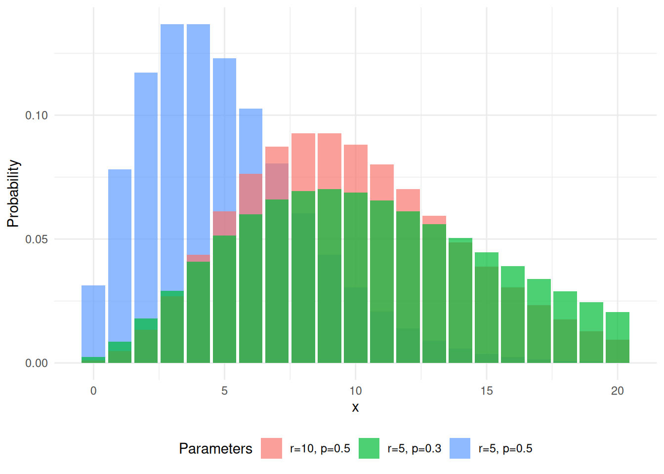
PMF \[ p_X(k) = \binom{k - 1}{r - 1}p^r\left(1 - p\right)^{k - r}\quad k = r, r+1, \dots \]
Expected Value
\[ \mathbb{E}\left[X\right] = \frac{r}{p} \]
Variance
\[ \operatorname{Var}\left[X\right] = r \frac{\left(1 - p\right)}{p^2} \]
A.5 Hypergeometric
The hypergeometric distribution models the number of successes in a sample drawn without replacement from a finite population containing a fixed number of successes. It is used in scenarios such as quality control or card games where the order of selection matters and the population is not infinite.
Distribution
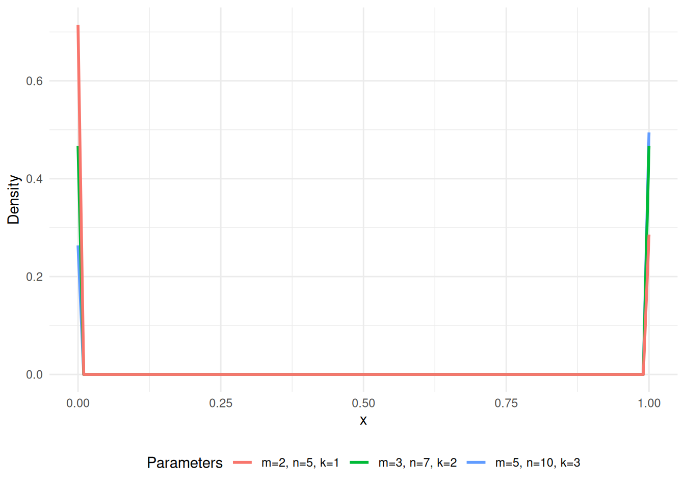
\[ \frac{\binom{m}{y} \binom{N - m}{n - y}}{\binom{N}{n}} \]
Expected Value
\[ \mathbb{E}\left[X\right] = n \cdot \frac{m}{N} \]
Variance
\[ \operatorname{Var}\left[X\right] = n \cdot \frac{m}{N} \cdot \left(1 - \frac{m}{N}\right) \cdot \frac{N - n}{N - 1} \]
A.6 Poisson
The Poisson distribution models the number of events occurring in a fixed interval of time or space, given that events occur independently at a constant average rate \(\lambda > 0\). It is often used for count data such as the number of arrivals per hour or defects per unit.
\(X \thicksim\operatorname{Po}\left(\lambda\right)\), \(\lambda > 0\), observations are independent, and \(\operatorname{log}\left(\lambda\right)\) is a linear function of \(x\).
Distribution
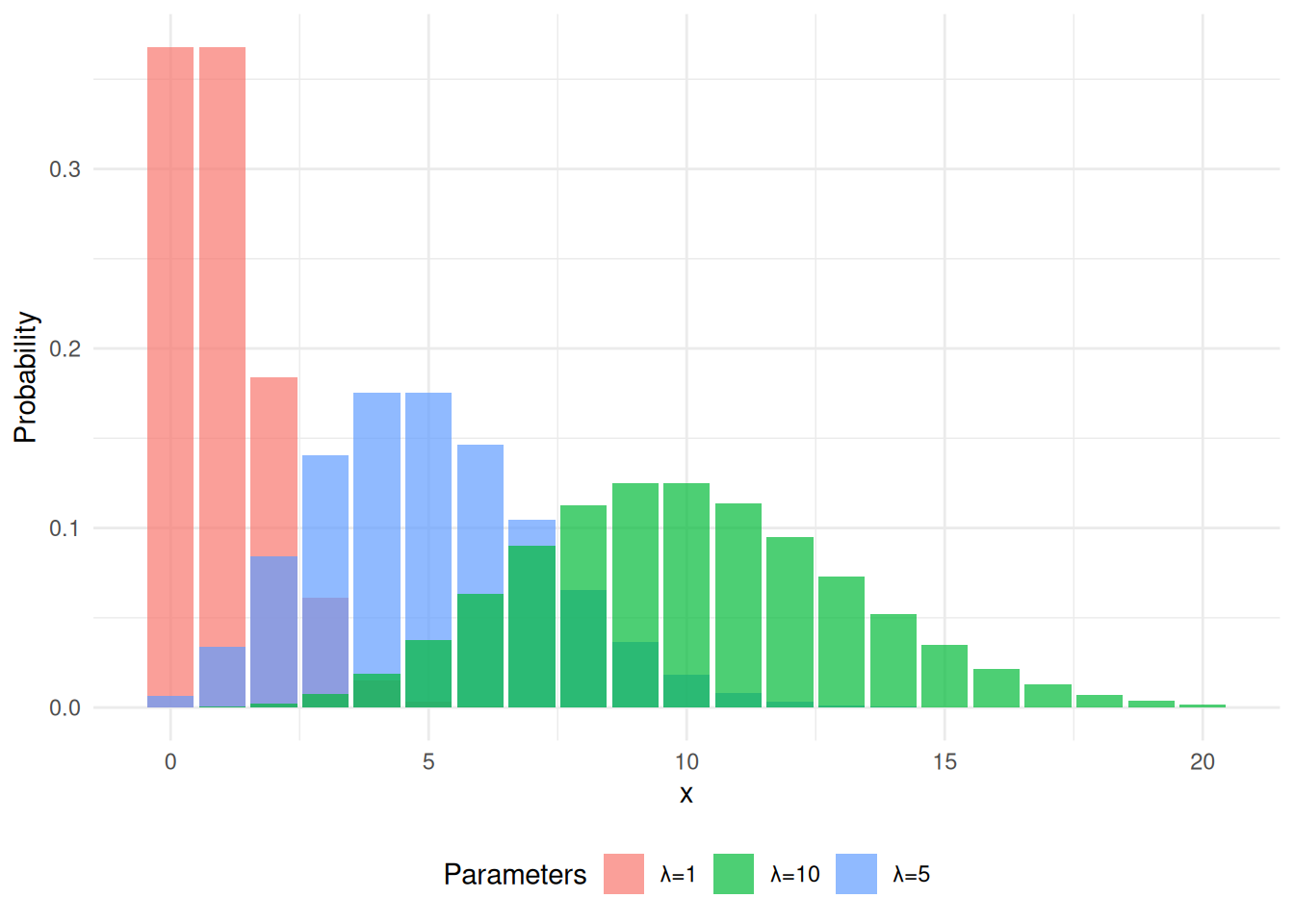
The PMF (see Section 2.1) is given as \[ p_X(x) = \frac{\lambda^x}{x!}\operatorname{exp}\left(-\lambda\right) \]
Expected Value
\[ \mathbb{E}\left[X\right] = \lambda \]
Variance
\[ \operatorname{Var}\left[X\right] = \lambda \]
A.7 Exponential
The exponential distribution models the time between events in a Poisson process, i.e., the waiting time until the next independent event occurs at a constant rate \(\lambda > 0\). It has the memoryless property: the probability of waiting an additional time \(t\) does not depend on how long one has already waited.
Distribution
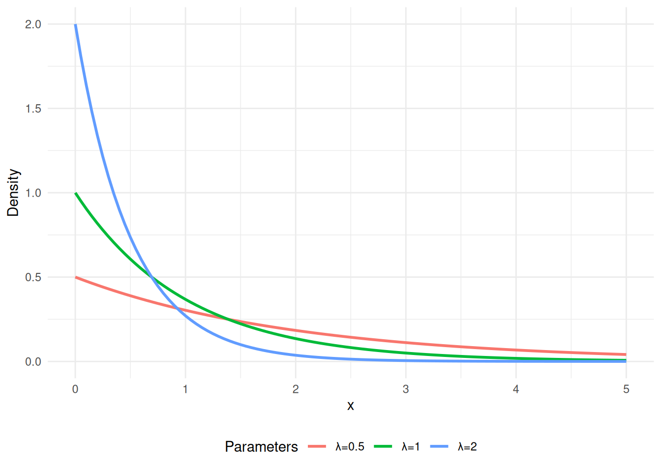
\[ f_X(x) = \begin{cases} \lambda \cdot \operatorname{exp}\left(-\lambda \cdot x\right) & x > 0 \\ 0 & x \leq 0 \end{cases} \]
Expected Value
\[ \mathbb{E}\left[X\right] = \frac{1}{\lambda} \]
Variance
\[ \operatorname{Var}\left[X\right] = \frac{1}{\lambda^2} \]
A.8 Gamma
The gamma distribution is a flexible two-parameter family of continuous distributions that generalizes the exponential distribution. It models the waiting time until the \(\alpha\)-th event in a Poisson process, and includes the chi-square and exponential distributions as special cases. \(X \thicksim\operatorname{Gamma}\left(\alpha, \beta\right)\), where \(\alpha > 0\) is the shape parameter and \(\beta > 0\) is the rate parameter.
Distribution
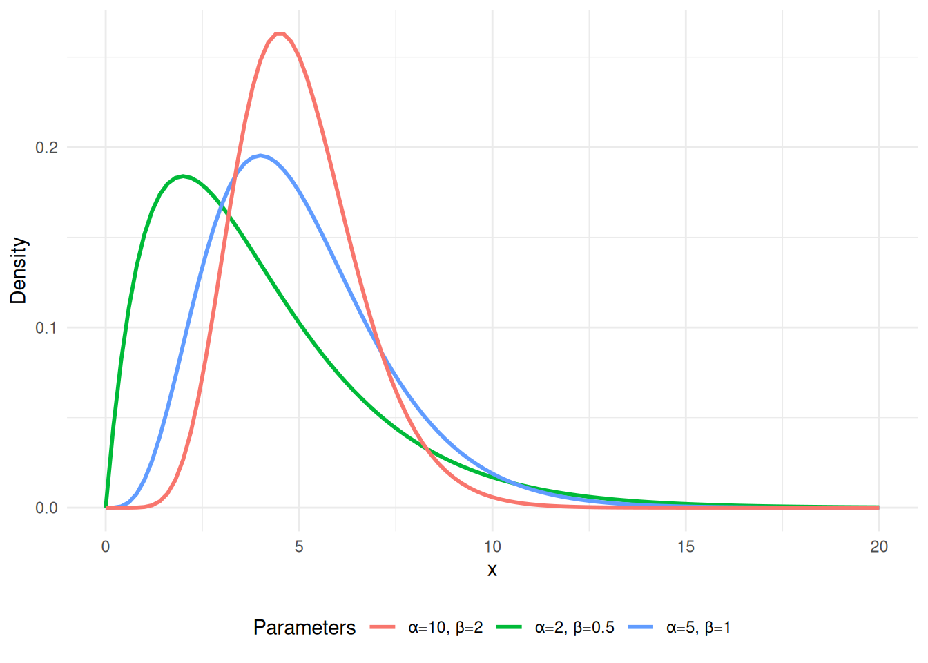
\(X \thicksim\operatorname{Gamma}\left(\alpha, \beta\right)\) \[ f_X(x) = \begin{cases} \frac{\beta^\alpha}{\varGamma(\alpha)} x^{\alpha - 1}\operatorname{exp}\left(-\beta \cdot x\right) & x > 0\\ 0 & x \leq 0 \end{cases} \]
Expected Value
\[ \mathbb{E}\left[X\right] = \frac{\alpha}{\beta} \]
Variance
\[ \operatorname{Var}\left[X\right] = \frac{\alpha}{\beta^2} \]
A.9 Gaussian
The Gaussian distribution is the most widely used continuous distribution, characterized by its symmetric bell-shaped curve. It arises naturally in many settings due to the central limit theorem, which states that sums of independent random variables tend toward a Gaussian distribution. \(X \thicksim\operatorname{N}\left(\mu, \sigma^2\right)\), with the standard Gaussian given as \(X \thicksim\operatorname{N}\left(0, 1\right)\).
Distribution
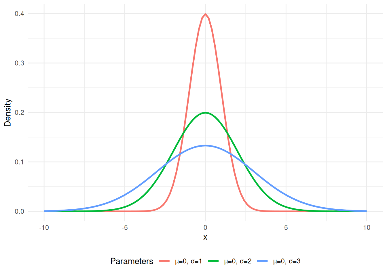
The PDF (see Section 2.3) is given as \[ f_X(x) = \frac{1}{\sqrt{2 \cdot \pi} \cdot \sigma} \cdot \operatorname{exp}\left(- \frac{1}{2 \cdot \sigma^2}\left(x - \mu\right)^2\right) \]
Expected Value
\[ \mathbb{E}\left[X\right] = \mu \]
Variance
\[ \operatorname{Var}\left[X\right] = \sigma^2 \]
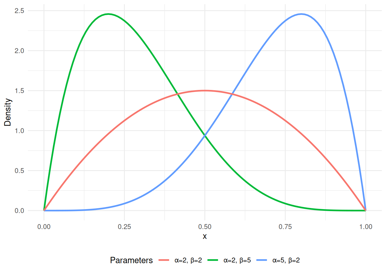
A.10 Beta
The beta distribution is a continuous distribution defined on the interval \([0, 1]\), making it well-suited for modeling probabilities or proportions. It is parameterized by two positive shape parameters \(\alpha\) and \(\beta\) that control the shape of the distribution, ranging from uniform to strongly skewed or U-shaped.
Distribution
Expected Value
\[ \mathbb{E}\left[X\right] = \frac{\alpha}{\alpha + \beta} \]
Variance
\[ \operatorname{Var}\left[X\right] = \frac{\alpha \beta}{(\alpha + \beta)^2 (\alpha + \beta + 1)} \]
A.11 Uniform
The uniform distribution assigns equal probability to all values within a bounded interval \([a, b]\). It is the simplest continuous distribution and is commonly used as a non-informative prior or for generating random samples via inverse transform sampling. \(X \thicksim\operatorname{U}\left(a, b\right)\).
Distribution
\[ f_X(x) = \begin{cases} \frac{1}{b - a} & x \in [a, b]\\ 0 & x \notin [a,b] \end{cases} \] \[ F_X(x) = \begin{cases} 0 & x < a\\ \frac{x - a}{b - a} & a \leq x \leq b\\ 1 & x > b \end{cases} \]
Expected Value
\[ \mathbb{E}\left[X\right] = \frac{1}{2}\left(a + b\right) \]
Variance
\[ \operatorname{Var}\left[X\right] = \frac{1}{12}\left(b - a\right)^2 \]
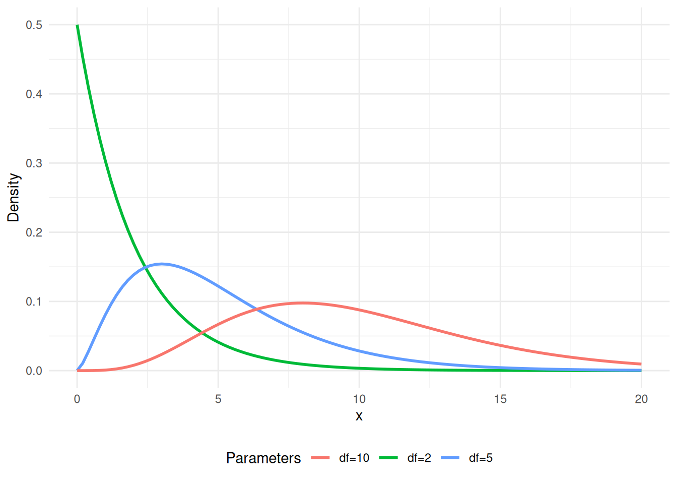
A.12 Chi-square
The chi-square distribution is a special case of the gamma distribution and arises as the distribution of the sum of squares of \(k\) independent standard Gaussian random variables. It is widely used in hypothesis testing (e.g., goodness-of-fit tests) and in the construction of confidence intervals for variance. \(X \thicksim\operatorname{Gamma}\left(\frac{k}{2}, \frac{1}{2}\right)\), \(k \in \mathbb{N}\).
Distribution
\[ f_X(x) = \begin{cases} \frac{x^{\frac{k}{2} - 1}\operatorname{exp}\left(-\frac{x}{2}\right)}{2^{\frac{k}{2} \cdot \varGamma\left(\frac{k}{2}\right)}} & x > 0 \\ 0 & x \leq 0 \end{cases} \]
Expected Value
\[ \mathbb{E}\left[X\right] = k \]
Variance
\[ \operatorname{Var}\left[X\right] = 2 \cdot k \]
A.13 F
Distribution
Expected Value
Variance
A.14 T
Distribution
\[ \frac{\Gamma\left(\frac{d + 1}{2}\right)}{\sqrt{\pi d} \cdot \Gamma\left(\frac{d}{2}\right)} \cdot \left(1 + \frac{x^2}{d}\right)^{-\frac{d + 1}{2}} \] \(d > 0\) is the degrees of freedom.
Expected Value
\[ \mathbb{E}\left[X\right] = \begin{cases} 0 & d > 1\\ \textrm{undefined} & d \leq 1 \end{cases} \]
Variance
\[ \operatorname{Var}\left[X\right] = \begin{cases} \frac{d}{d - 2} & d > 2 \\ \infty & 1 < d \leq 2 \\ \textrm{undefined} & d \leq 1 \end{cases} \] $$